To get column totals of a range that contain numeric values, use the TOTALCOL function or a custom formula that uses the MMULT function.
This tutorial will show various methods to get column totals from a selected range. First, we introduce the TOTALCOL function, the simplest way to return column totals. In the second part of the article, we will write formulas that use regular Excel functions.
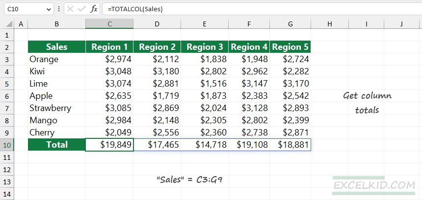
How to get column totals of a range?
- Type the =TOTALCOL(C3:G9) formula in cell C10.
- Press Enter.
- The formula sums each column in the selected range.
Syntax
=TOTALCOL(range)Arguments
The TOTALCOL function uses a single, required argument, the range where we find the columns.
Example
In the example, the data is in the range C3:G9. Next, select the range of cells, click the name box, and add a descriptive name to a range, for example, “Sales”. From now on, “Sales” refers to the range C3:G9.
Formula:
=TOTALCOL(sales)The formula returns the sum of each column in the selected range.
Note: TOTALCOL is a dynamic array function, that is mean the result spills into a range. The function is compatible with Excel 2010 up to the latest Microsoft 365 versions. So if you are working with Excel 2010, 2013, 2016, or 2019, press Ctrl+Shift+Enter to create the result array.
Get column totals using the MMULT function
To get column totals from a range, you can use matrix multiplication. To do that, apply the MMULT function that uses two arrays as input and generates a return array with the following conditions: the output array has the same number of columns as the first array. It uses the same number of rows as the second.
The formula in C10:
=MMULT(TRANSPOSE(ROW(Sales)^0),--Sales)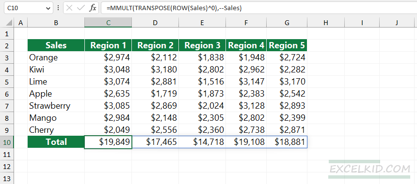
The MMULT function needs a numeric input, so we use a double negative (–) to fill the array with zero instead of empty cells.
In the example, array2 contains 7 rows; the formula needs array1, which includes 5 columns. The result should be a 1×7 array since the result spills into the range C10:G10.
=TRANSPOSE(ROW(data)^0)As a result of the formula, the ROW function returns a 1×7 array that contains row numbers:
=ROW(Sales) = {3, 4, 5, 6, 7, 8, 9}
=ROW({3, 4, 5, 6, 7, 8, 9)} = {1, 1, 1, 1, 1, 1, 1}
TRANSPOSE converts the horizontal array to vertical, from 7×1 to 1×7; we will use the result as array1 for the MMULT function. Finally, the MMULT multiplicates the two arrays and gets column totals.
Using the SEQUENCE function
Another method to create an array input for the MMULT function is to use the SEQUENCE function.
Formula:
=MMULT(SEQUENCE(1,ROWS(Sales),1,0),--Sales)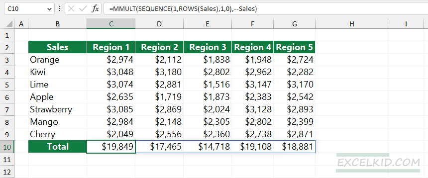
In this case, you do not need to use the TRANSPOSE function; the formula returns the column totals.
=SEQUENCE(1,ROWS(Sales),1,0)