Use the Excel COMPARE function to compare two lists or ranges and extract values based on different aspects.
If you are working with ranges in Microsoft Excel, sometimes you compare two columns and extract matches and differences. You can write various Excel formulas to get the common values from two lists.
Today we will introduce the Excel COMPARE function. With its help, you can create short formulas for comparison purposes.
COMPARE Function
Syntax
=COMPARE(list1,list2)Arguments
The COMPARE function uses two required and one optional argument.
- rng1 = range1 is the first range you want to compare
- rng2 = range2 is the second range you want to compare
- returnType = optional argument, control the calculation
Examples
Using the function, you can perform three types of calculations:
- If you use only the first two required arguments (or set the argument to 0), the function compares two ranges and returns the common records. You can compare any data type, for example, text or numeric values.
- Set the 3rd argument to 1; the function will return an array of values that exists in range1 and not in range2.
- Set the 3rd argument to 2; the function will return an array of values that exists in range2 and not in range1.
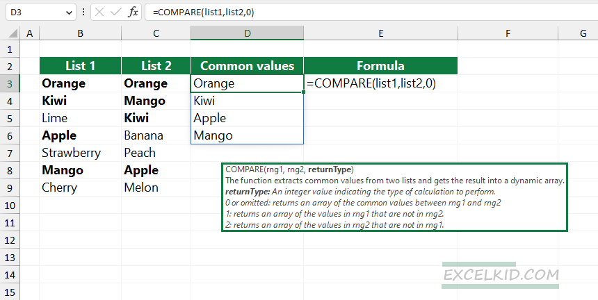
To get the common values, use the following formula; you can use only the required arguments. Type the formula in cell D3. The values that appear in both lists spill into the range D3:D6.
=COMPARE(list1, list2)Formula to get only these values that appear in list1 but not in list2:
=COMPARE(list1, list2, 1)Formula to get only these values that appear in list2 but not in list1:
=COMPARE(list1, list2, 2)As you see, using the COMPARE function, you can save a lot of work. To get more time-saving functions, check our free add-in, DataFx, which supports 200 user-defined functions.
Additional resources: