
Our definitive guide will show you 15 ways to clean data in Excel. Learn more about data cleansing through useful examples.
Clean data and string manipulation formulas in Excel are critical! Besides the well-known techniques, we will introduce special VBA codes to make the process quicker and more effective.
Table of contents:
- Sorting data to check extremes and peaks
- Remove duplicates to clean data
- Use the find and replace function
- Check the type of data in a cell
- Convert numbers stored as text into numbers
- Eliminate blank cells in a list or range
- Clean data using split the text into columns
- Concatenate text using the TEXTJOIN function
- Change text to lower – upper – proper case
- Remove non-printable characters using the CLEAN formula
- Remove unnecessary characters from text automatically
- Clean extra spaces using the TRIM function
- Insert text after specific nth characters
- Delete the text after the nth character
- Remove special characters from a text
Introduction to Data Cleansing in Excel
Data cleansing is Excel, not just a task; it is an art that turns raw data into a masterpiece of insights and information. The path to learning this art begins with understanding the foundation: Excel. Our guide does not just walk you through the fundamental steps; it searches into the lesser-known methods, revealing 15 effective ways to clean your data. We introduce a world where Excel’s string manipulation formulas and VBA codes become your friends in the battle against data clutter. We will show you special VBA codes that accelerate the cleansing process, making it effective and efficient.
Imagine the satisfaction of filtering through millions of data points to identify the outliers or the aid when you remove duplicates with a simple click, ensuring a clean dataset. We will explain multiple scenarios with practical examples, demonstrating the power of Excel’s functions – like ‘Sort’, ‘Text to Columns’, ‘TRIM’, and the ‘CLEAN’ formula.
But the tutorial is not just about cleaning what is visible. It goes beyond addressing the invisible threats like non-printable characters and excess spaces that lurk within your sheets, waiting to undermine your analysis. Moreover, we tell a personal story and provide tips that make the journey through data cleansing a learning adventure. It is about transforming a boring task into an opportunity to explore the full potential of your data.
Finally, we introduce our Excel add-in, DataXL, transforming complex string manipulations into a child’s play.
Effective ways to clean data in Excel
Let us see the basics first! Sometimes, the best method is the “back to the roots” and starts the data cleansing project with simple but effective solutions.
Prologue
Before we take a deep dive into this topic, allow us to tell a personal story.
After college, I worked at a small company with limited HR resources. As newbies, they didn’t dish out the easy tasks for me. Okay, let’s clean the data in Excel. I got countless boring tasks. The main issue was how to create clean data just in time. I had never heard of the Excel string manipulation functions, so the solution wasn’t simple – many night shifts; good, old days.
After that, we formed our own company and worked on various plans. Finally, we had enough resources to develop a powerful Excel add-in for data cleansing.
We aim to make text manipulation and Excel data processing a child’s play for you. So today, we publish a universal Excel add-in tool. From now on, string manipulation and data cleansing will be easy! Read more about the utility.
#1 – Sorting data to check extremes and peaks
Is it possible to find errors in a list using simple sorting? Yes! We have nothing to do but arrange the data in a growing or decreasing order. Right-click on the cell and choose the ‘Sort Largest To Smallest’ option from the menu. Seldom can there be found extremely small or large, maybe peeking data?
Look at the picture below:
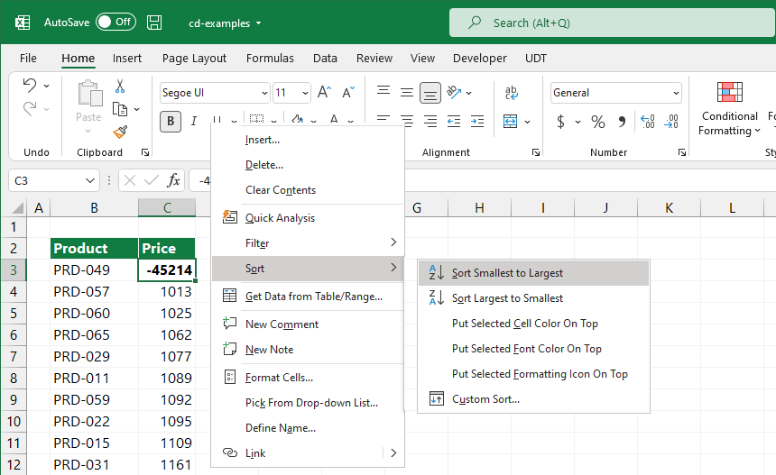
Who would ever think you could find these mistakes in several million records? Alternatively, conditional formatting can find errors and blanks in a range.
#2 – Remove duplicates to clean data
Excel supports many options to eliminate duplicates. For example, two tightly joined operations filter unique values and remove duplicated data. The result is the same in both cases: a list of unique values.
To filter for unique values (filtered list), use the Advanced command on the Data tab in the Sort & Filter group.
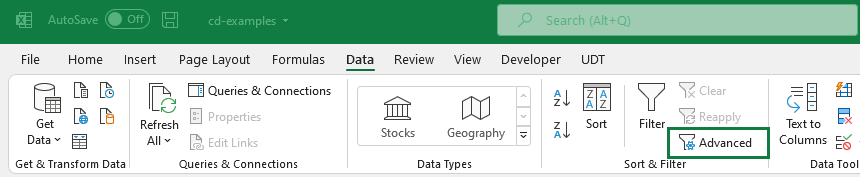
Select the range of cells! Then go to the Data tab! In the Sort & Filter group, click Advanced. Next, choose the Unique records only check box and click OK.
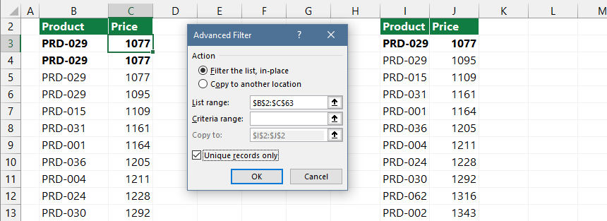
Explanation: However, there is one significant difference that we cannot ignore. In the process of filtering unique values, it temporarily hides the duplicated values. You can go back to your original list to undo this operation.
You’ll permanently delete duplicates using the ‘Remove Duplicates’ tool on the ribbon! Pay attention to this! The removed, deleted items will last after saving the Workbook. So be very careful.
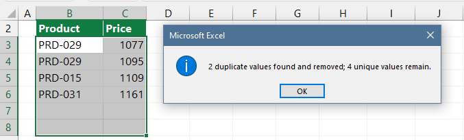
Let us see how the duplicate removal values tool works! First, select the range. Then, go to the Data tab! Then, in the Data Tools group, click Remove Duplicates.
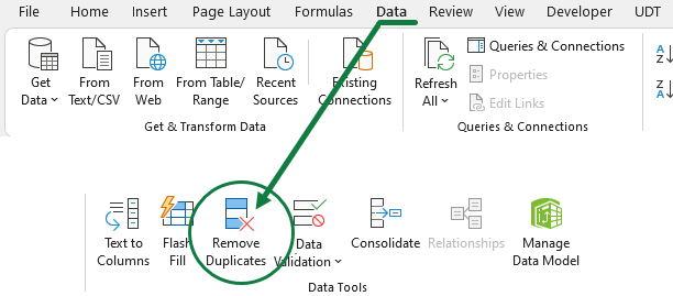
Select one or more columns, then click OK. A message box will appear and shows how many duplicated values are removed and how many unique ones remain.
Finally, read this definitive guide to learn more about removing duplicates.
#3 – Use the find and replace function
The advantage of the Find & Replace function is that we can work with it relatively fast in any size data table. First, let’s see how to clean data using this function. To find and replace data in a worksheet, follow these steps:
Press the Ctrl+H keyboard shortcut, and the Find and Replace dialog box appears.
In the Find What box, enter the data you want to locate. Then, enter the Replace With box the data you want to replace.
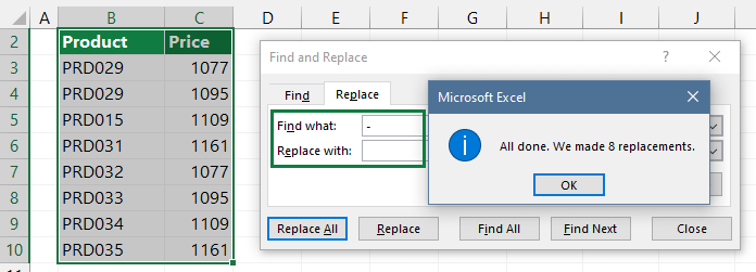
If you want to replace all occurrences simultaneously, click Replace All.
#4 – Check the Type of Data in a Cell
Please wait a minute before we make any changes to the raw data.
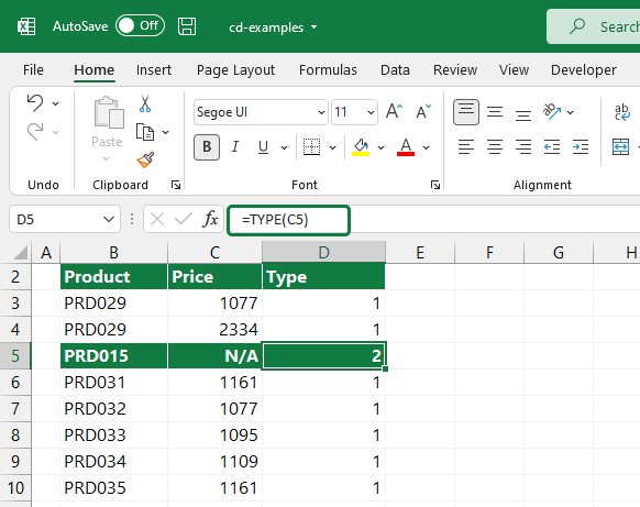
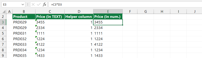
We have to check the type of data in the cell. We can do this by using the TYPE function. The function is one of a group of information functions. Numeric or text data? In the picture below, you can see what kind of results the formula brings in the case of different types of data.
If the function returns 1, the data type is numeric. If it’s returning with 2, the data type is text.
#5 – Convert Numbers Stored as Text into Numbers
If we import data from a text file or an external data source into Excel, Excel often stores numbers as text. It can be the source of many problems, but there are ways to avoid mistakes.
Create a helper column and type 1. Next, apply a simple multiply using this formula: number (stored as text) * 1. A result is a number.
Read more about how to convert text to numbers.
#6- Eliminate blank cells in a list or range
Now we’ll highlight the whole range that also contains the empty lines. Press the F5 key, and choose the ‘Special’ option from the popup window.
All the cells in the selected range that are not blank are deselected, leaving only the blank cells selected.
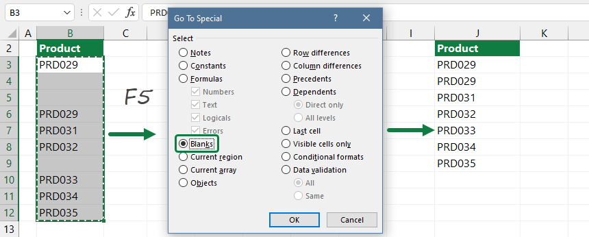
Click ‘Delete‘ in the ‘Cells’ section of the ‘Home‘ tab.
Finally, select ‘Delete Sheet Rows‘ from the drop-down menu.
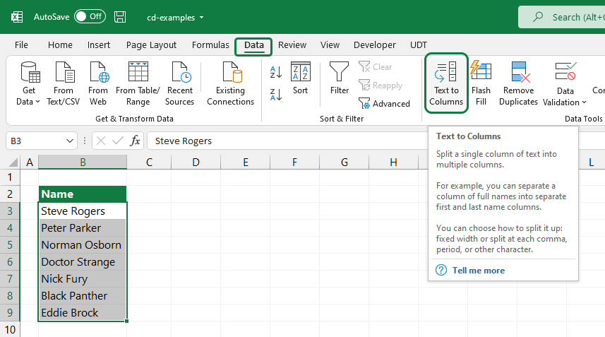
#7 – Split text into columns
It’s easy to split text into multiple cells. For example, suppose that our data set contains our clients’ first and family names in one cell. We want to split the names so that the first names and family names are in different columns.
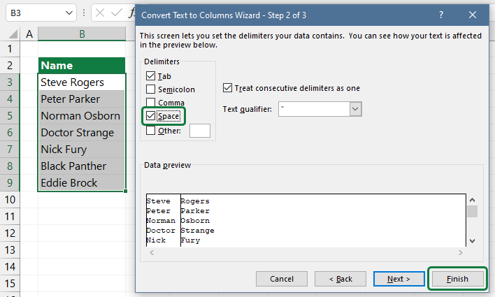
Start the ‘Convert Text to Columns Wizard’ and follow the steps below:
First, select the range that contains names. Next, click Text to Columns in the Data Tools group.
Select the Delimiters checkbox and click Next.
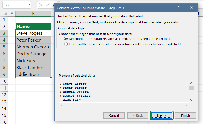
Leave all the checkboxes empty under the Delimiters section. Now check the Space check box (in our example). Click Finish!
#8 – Concatenate text using the TEXTJOIN function
Let’s see the opposite of the previous section. Now, we want to combine the text from several cells into one. How can we solve this problem quickly?
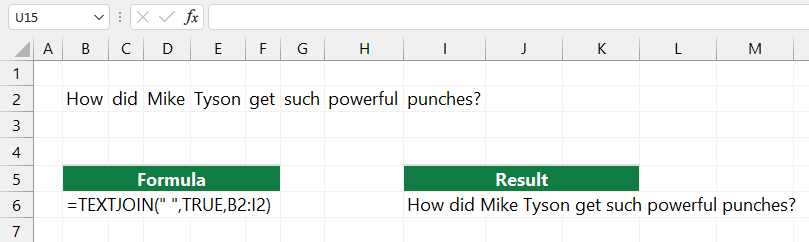
The TEXTJOIN function joins (what a surprise) values using a selected delimiter. It provides better functionality than CONCAT. This function allows you to supply a range of cells and has a setting to ignore empty values.
Take a look at the formula bar! You can use space as a delimiter. The second parameter is TRUE because we want to ignore the empty cells (if available).
If you are using an earlier version of Excel, you should install 3rd party add-in.
#9 – Change Text to Lower – Upper – Proper Case
Let’s see what kind of Excel text transformation formulas we can use to transform the text. It is worth using them during data cleansing.
- LOWER() transforms the given text into lowercase letters. Example: LOWER(‘EXCEL’), result: ‘excel’
- UPPER() changes the given text into upper case letters. Example: UPPER(‘excel’), result: ‘EXCEL’
- PROPER() transforms the first letter of the character string and the letters standing after non-letters into upper case letters.
Example:
=PROPER(‘Information is BEAUTIFUL’)
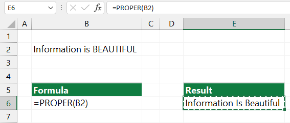
The result of the conversion is: ‘Information Is Beautiful. Not too often, but we might use these kinds of transformations also.
#10 – Remove non-printable characters – The CLEAN formula
Removing non-printable characters is one of the most advanced parts of data cleansing! We can say that work is relatively complex with special text formulas. We have made some short VBA codes for several possibilities.
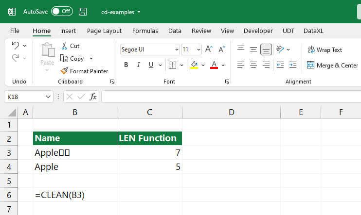
The non-printable Unicode characters are 129, 141, 143, 144, and 157.
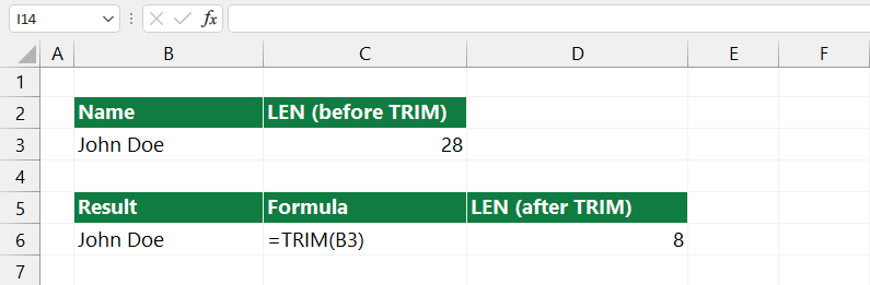
Let’s see how it works with the help of the following example. The text in cell B3 contains non-printable characters. So, first, you can check the result using LEN() formula. Then, to remove the unnecessary text parts, use the CLEAN function.
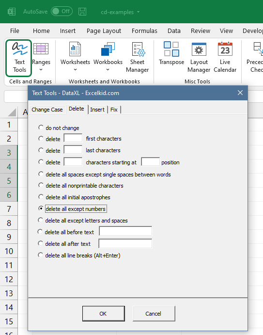
#11 – Remove unnecessary characters from text automatically
If we only want to delete special characters, the following tool can help. Download our add-in to remove alpha, numeric, or non-numeric characters in seconds.
#12 – Clean extra spaces using the TRIM function
Removing extra spaces from the text needs more attention.
You can find spaces at the beginning, middle, or end of the text. The hardest to recognize is the letter ones because they are invisible to the naked eye.
We’ll explain the two reasons they have to be removed. First, they can cause mistakes in the use of formulas. Imagine, for example, that the result of the VLOOKUP() formula is incorrect. It may sound funny, but it is not. Some formula mistakes may influence the outcome of the final calculation.
The other reason is the size of the file. However, indeed, the one-character surplus is not baneful. Problems occur when the Excel database contains several million records.
Yes, there are some like this. Just think about the external data sources and Power Query output. In this case, the size increase can be 5% – 10%. We don’t have to depict the harmful effects of this. Use the TRIM() formula and guarantee that the list will be clean.
#13 – Insert text after specific nth characters
Using some Excel functions, we can resolve that we insert some characters in front of or behind a given string. The problem starts when we perform this operation on an Excel database.
We can manipulate massive data sets in seconds by choosing the ‘Text Tools’ option! However, executing this task manually is challenging if you use simple Excel formulas.
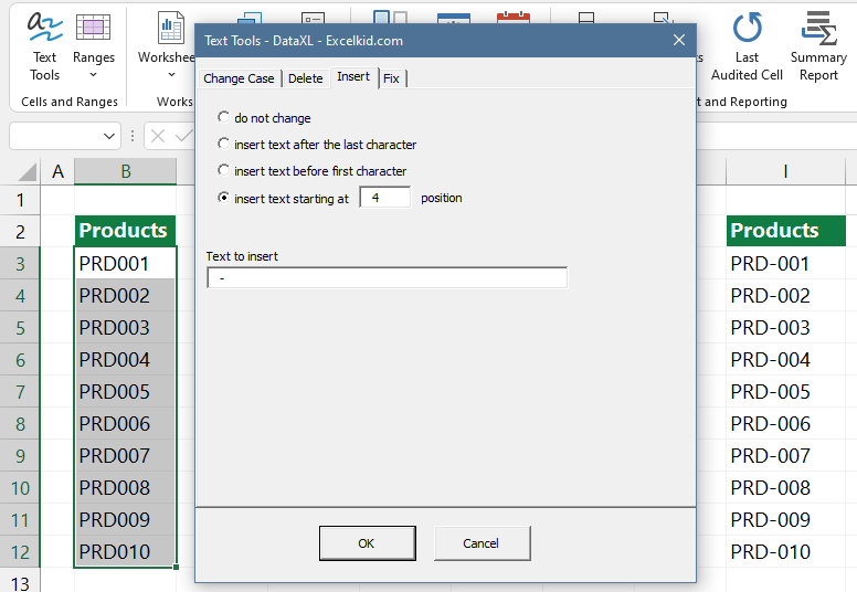
From the Excel string manipulation formulas, we have to emphasize the SEARCH(), FIND(), MID(), LEFT(), and RIGHT() functions.
Imagine that comfortable situation where you don’t have to create endless formulas again! Instead, start the functions that you can see in the picture.
#14 – Delete the text after the nth character
The following data cleansing task is a real threat to Excel users. Let’s stay a little longer with the string manipulation functions. Opposite to the previous paragraph, we don’t insert the characters but remove them.
At this point, all people who are good at Excel would say: Let’s cut the characters from the front and back. What if we do this from the middle of the text or starting from the fifth character?
Probably, this is the moment when the average user would throw the keyboard from the desk.
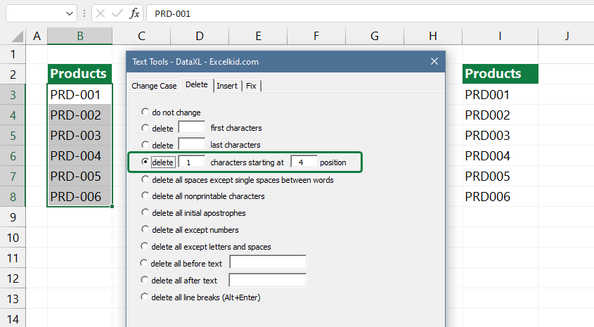
Please try the remove-by-position function; it is a very effective working tool. Then, look through the list. The result will quickly restore your blood pressure.
#15 – Remove special characters from a text
Finally, let’s see the special characters. We distinguish three different types. The first is the non-printable characters, the second is the alpha characters, and the third is the numerical data. The tools seen in the picture can remove only one type of character from the text.
Imagine how useful can be this Excel application if we have to cleanse a database containing phone numbers. The cells have numbers and other characters.
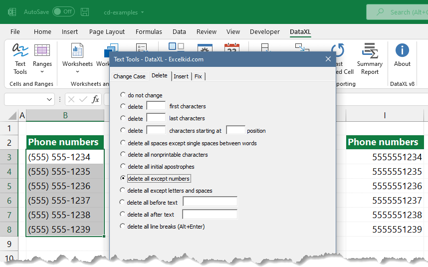
Let’s say we need data that only can contain numbers. And the list of phone numbers has five thousand rows. What do you think about how long would it take to remove the hyphens and other non-numerical characters? It takes too long, only thinking about it! Use Excel and automated data-cleaning functions! The execution time narrows down to seconds. It looks great!
Enhance Your Excel Data Cleansing Skills with Real-World Applications
In the ever-evolving landscape of data analysis, the ability to clean and refine your data stands out as a pivotal skill that can significantly enhance the quality of your insights and the efficacy of your decision-making processes. Recognizing this, we have meticulously crafted resources that not only elucidate the theoretical aspects of data cleansing in Excel but also provide you with practical tools to apply these concepts effectively.
Dive Deep Into Real-World Success with Our Case Studies
Our collection of case studies serves as a beacon for all data enthusiasts, shedding light on the transformative impact of proficient data cleansing. These stories from the business world offer a vivid glimpse into how organizations, just like yours, have navigated the complexities of raw data to uncover valuable insights that drive strategic decisions and operational efficiencies. By exploring these case studies, you will gain not only inspiration but also practical strategies that can be adapted to your own data challenges, regardless of the industry.
Sharpen Your Skills with Hands-On Data Cleansing Projects
To complement the theoretical knowledge and real-world examples, we have prepared an exclusive set of Sample Data Cleansing Projects. These downloadable Excel files are your playground for experimentation, offering a variety of scenarios that challenge and refine your data-cleansing skills. From beginners to advanced users, these projects are designed to cater to all levels, enabling you to practice and perfect the techniques discussed in our guide. You’ll learn to navigate through common data quality issues, apply sophisticated cleansing methods, and ultimately, transform your data into a clean, analysis-ready format.
Your Path to Becoming a Data Cleansing Expert
As you embark on this journey, remember that the road to mastering data cleansing in Excel is both rewarding and continuous. The skills you develop will not only improve your immediate data analysis tasks but also set a foundation for advanced data management techniques. We encourage you to leverage these case studies and sample projects as stepping stones towards becoming a confident and competent data analyst.
Join a Community of Data Enthusiasts
But your journey doesn’t have to be a solitary one. We invite you to join our community of data enthusiasts where you can share your experiences, challenges, and triumphs in data cleansing. Whether through forums, social media groups, or our comment sections, engaging with peers can provide additional insights, motivate you to tackle complex data issues, and keep you updated on the latest Excel features and data management trends.
Continual Learning and Improvement
Lastly, we understand that the landscape of data and Excel is constantly evolving. As such, we commit to updating our resources, case studies, and project files to reflect the latest advancements and best practices in the field. Keep an eye on our platform for updates, and don’t hesitate to reach out with your feedback or suggestions for new content.
By embracing these resources, engaging with the community, and committing to continual learning, you are on your way to unlocking the full potential of your data with Excel. Transform raw data into insightful, clean datasets that can inform your most critical decisions and propel your projects or organization forward.
Final Thoughts: Use Effective Methods to Clean Data in Excel
Let’s summarize what we have learned today! We have introduced the most important text transformations and their field of use. The free data cleansing add-in will take a lot of weight off your shoulders. To increase your knowledge of Excel, visit the well-known Excel forums.
There is no shame in learning from professionals. That’s what we have done in the early days. However, excel string manipulation functions are a huge subject that needs time and attention. As we can see from the article, Excel offers many possibilities to improve data quality.
Some functions we made with VBA macros; you should check these out closely. We hope that you will create a flawless analysis with the help of the introduced data cleansing techniques.
Additional resources: